Partitioning

Introduction

Oracle Partitioning, first introduced in Oracle 8.0 in 1997, is one of the most important and successful functionalities of the Oracle DB, improving the performance, manageability, and availability for tens of thousands of applications. 

11gR2 introduces the 9th generation of partitioning, enabling customers to model even more business scenarios and making partitioning easier to use, enabling “Partitioning for the masses”.

Partitioning allows a table, index, or index-organized table to be subdivided into smaller pieces called partitions using single or set of columns called partitioning key. For ex, orders table can be partitioned based on order_date as partitioning key. Each piece of such a DB object is called a partition. Each partition has its own name, and may optionally have its own storage characteristics. 

Basics of Partitioning

• Partitioning addresses key issues in supporting very large tables and indexes by decomposing them into smaller and more manageable pieces called partitions, which are entirely transparent to an application.
• SQL queries and DML statements do not need to be modified to access partitioned tables. However, after partitions are defined, DDL statements can access and manipulate individual partitions rather than entire tables or indexes. This is how partitioning can simplify the manageability of large database objects.
• Each partition of a TABLE / INDEX must have the same logical attributes, such as column names, data types, and constraints, but each partition can have separate physical attributes, such as compression enabled or disabled, physical storage settings, and tablespaces.
• Database objects - tables, indexes, and index-organized tables - are partitioned using a 'partitioning key', a set of columns that determine in which partition a given row will reside.
• However, the DBA can manage and store each monthly partition individually, potentially using different storage tiers, applying table compression to the older data, or store complete ranges of older data in read only tablespaces.
• From the perspective of a DBA, a partitioned object has multiple pieces that can be managed either collectively / individually. This gives the DBA considerable flexibility in managing a partitioned object. 
• From the perspective of the Application, a partitioned table is identical to a non-partitioned table; no modifications are necessary when accessing a partitioned table using SQL DML commands.
• Note: All partitions of a partitioned object must reside in tablespaces of a single block size.

Partitioning Key: Each row in a partitioned table is unambiguously assigned to a single partition. Partitioning key consists of one or more columns that determine the partition where each row is stored. Oracle automatically directs insert, update, and delete operations to the appropriate partition with the partitioning key.

Partitioned Tables: Any table can be partitioned into a million separate partitions except those tables containing columns with LONG / LONG RAW data types. You can, however, use tables containing columns with CLOB / BLOB data types.

Partitioned Index-Organized Tables: They are very useful for providing improved performance, manageability, and availability for index-organized tables. For partitioning an index-organized table:

• Partition columns must be a subset of the primary key columns.
• Secondary indexes can be partitioned (both locally and globally).
• OVERFLOW data segments are always equi-partitioned with the table partitions.

Exactly, when to use partitioning is a rather subjective decision. Some general guidelines that Oracle and I suggest are listed below.

When to Partition a Table

• Tables greater than 2 GB should always be considered as candidates for partitioning.
• Tables containing historical data, in which new data is added into the newest partition. A typical ex. is a historical table where only the current month's data is updatable and the other 11 months are read only.
• When the contents of a table need to be distributed across different types of storage devices.

When to Partition an Index

• Avoid rebuilding the entire index when data is removed.
• Perform maintenance on parts of the data without invalidating the entire index.
• Reduce the impact of index skew caused by an index on a column with a monotonically increasing value

Benefits of Partitioning

• It enables the DB objects to be managed and accessed at a finer level of granularity. 
• It improves the performance of certain queries or maintenance operations by an order of magnitude. 
• It can greatly reduce the total cost of data ownership, using a “tiered archiving” approach of keeping older relevant information still online on low cost storage devices.
• It enables an efficient and simple, yet very powerful approach when considering Information Lifecycle Management (ILM) for large environments.
• It also enables DB designers and DBA's to tackle some of the toughest problems posed by cutting-edge applications. 
• It is a key tool for building multi-terabyte systems or systems with extremely high availability requirements.
• It can provide tremendous benefit to a wide variety of applications by improving Performance, Manageability, and Availability. 

Partitioning for 

• Availability: Partitioned DB objects provide partition independence. This characteristic of partition independence can be an important part of a high-availability strategy.
• Manageability: It allows tables and indexes to be partitioned into smaller, more manageable units, providing DBA with the ability to pursue a "divide and conquer" approach to data management.
• Performance: By limiting the amount of data to be examined / operated on, partitioning provides a number of performance benefits. These features include: Partitioning Pruning and Partition-wise Joins.

Oracle additionally provides a comprehensive set of SQL commands for managing partitioning tables. These include commands for adding new partitions, dropping, splitting, moving, merging, truncating, and optionally compressing partitions.

Partitioning Pruning / Partition Elimination

• It is the simplest and also the most substantial means to improve performance using partitioning. Partition pruning can often improve query performance by several orders of magnitude.
• In Partition Pruning, the optimizer analyzes FROM and WHERE clauses in SQL statements to eliminate unneeded partitions when building the partition access list. As a result, Oracle DB performs operations only on those partitions that are relevant to the SQL statement. Partition pruning dramatically reduces the amount of data retrieved from disk and shortens processing time, thus improving query performance and optimizing resource utilization.
• Partition pruning works with all of Oracle's other performance features. Oracle will utilize partition pruning in conjunction with any indexing technique, join technique, or parallel access method. 

 Partition-wise Joins

• It breaks a large join into smaller joins that occur between each of the partitions, completing the overall join in less time. It can be applied when two tables are being joined together, and at least one of these tables is partitioned on the join key or when a reference partitioned table is joined with its parent table.
• It reduces query response time by minimizing the amount of data exchanged among parallel execution servers when joins execute in parallel. This significantly reduces response time and improves the use of both CPU and memory resources. Partition-wise joins can be Full or Partial. Oracle DB decides which type of join to use.
• It break a large join into smaller joins of “identical” data sets for the joined tables. “Identical” here is defined as covering exactly the same set of partitioning key values on both sides of the join, thus ensuring that only a join of these 'identical' data sets will produce a result and that other data sets do not have to be considered.
• Oracle is using either the fact of already (physical) equi-partitioned tables for the join or is transparently redistributing (= “repartitioning”) one table at runtime to create equi-partitioned data sets matching the partitioning of the other table, completing the overall join in less time. This offers significant performance benefits both for serial and parallel execution.

Evolution of Partitioning in Oracle

Oracle Version #	Core functionality	Performance	Manageability
8	Range partitioning Global range indexes	“Static” partition pruning	Basic maintenance operations: add, drop, exchange
8i	Hash partitioning Composite range-hash partitioning	Partition-wise joins “Dynamic” pruning	Merge operation
9i	List partitioning		Global index maintenance
9i R2	Composite range-list partitioning	Fast partition split
10g	Global hash indexes		Local index maintenance
10g R2	1M partitions per table	“Multi-dimensional” pruning	Fast drop table
11g	More composite choices REF partitioning Virtual column partitioning		Interval partitioning Partition Advisor

Partitioning Strategies in 11g R2

Each partitioning strategy has different advantages and design considerations. Thus, each strategy is more appropriate for a particular situation.

Basic Partitioning Strategies		Partitioning Extensions
Single-level partitioning Range Hash List	Composite partitioning Range-Range Range-Hash Range-List Hash-Range Hash-Hash Hash-List List-Range List-Hash List-List	Manageability Extensions Interval Partitioning Interval Interval-Range Interval-List Interval-Hash Partition Advisor Partitioning Key Extensions REF Partitioning / Partition by Reference Virtual column-based Partitioning

Partitioning Strategies	Data Distribution	Sample Business Case
Single-level partitioning	Based on consecutive ranges of values Based on unordered lists of values Based on a hash algorithm	Orders table range partitioned by order_date Orders table list partitioned by country Orders table range partitioned by customer_id
Composite partitioning	Based on a combination of two of the above mentioned basic techniques of Range, List, Hash, and Interval	Orders table is range partitioned by order_date and sub_partitioned by hash on customer_id range on shipment_date
Interval partitioning	An extension to Range Partition. Defined by an interval, providing equi-width ranges. With exception of the first partition all partitions are automatically created on-demand when matching data arrives.	Orders table partitioned by order_date with a predefined daily interval, starting with '01-Jan-2012'
REF Partitioning or Partition by Reference	Partitioning for a child table is inherited from the parent table through a primary key - foreign key relationship. The partitioning keys are not stored in actual columns in the child table.	(parent) Orders table range partitioned by order_date and inherits the partitioning technique to (child) order lines table. Column order_date is only present in the parent orders table
Virtual column-based partitioning	Defined by one of the above mentioned partition techniques and the partitioning key is based on a virtual column. Virtual columns are not stored on disk and only exist as metadata.	Orders table has a virtual column that derives the sales region based on the first three digits of the customer account number. The orders table is then list partitioned by sales region.

Single-Level Partitioning: A table is defined by specifying one of the following data distribution methodologies, using one or more columns as the partitioning key:

1. Range: It maps data to partitions based on ranges of values of the partitioning key that you establish for each partition. It is the most common type of partitioning and is often used with dates.
2. List: It enables you to explicitly control how rows map to partitions by specifying a list of discrete values for the partitioning key in the description for each partition. The advantage of list partitioning is that you can group and organize unordered and unrelated sets of data in a natural way.
3. Hash: It maps data to partitions based on a hashing algorithm that Oracle applies to the partitioning key that you identify. Hashing algorithm evenly distributes rows among partitions, giving partitions approximately the same size.

Composite Partitioning: It is a combination of the basic data distribution methods; a table is partitioned by one data distribution method and then each partition is further subdivided into subpartitions using a second data distribution method. It supports historical operations, such as adding new range partitions, but also provides higher degrees of potential partition pruning and finer granularity of data placement through subpartitioning.

1. Range-Range: It enables logical range partitioning along two dimensions; for example, partition by order_date and range subpartition by shipping_date.
2. Range-Hash: It partitions data using the range method, and within each partition, subpartitions it using the hash method. Composite range-hash partitioning provides the improved manageability of range partitioning and the data placement, striping, and parallelism advantages of hash partitioning.
3. Range-List: It partitions data using the range method, and within each partition, subpartitions it using the list method. Composite range-list partitioning provides the manageability of range partitioning and the explicit control of list partitioning for the subpartitions.
4. List-Range: It enables logical range subpartitioning within a given list partitioning strategy; for example, list partition by country_id and range subpartition by order_date.
5. List-Hash: It enables hash subpartitioning of a list-partitioned object; for example, to enable partition-wise joins.
6. List-List: It enables logical list partitioning along two dimensions; for example, list partition by country_id and list subpartition by sales_channel.

Manageability Extensions: The following extensions significantly enhance the manageability of partitioned tables

Interval Partitioning: It is an extension of range partitioning which instructs the DB to automatically create partitions of a specified interval when data inserted into the table exceeds all of the existing range partitions. Range partitioning key value determines the high value of the range partitions, which is called the transition point, and DB creates interval partitions for data with values that are beyond that transition point. 

   When using interval partitioning, consider the following restrictions:

• You can only specify one partitioning key column, and it must be of NUMBER or DATE type.
• Interval partitioning is not supported for index-organized tables.
• You cannot create a domain index on an interval-partitioned table.

   You can create single-level interval partitioned tables and the following composite partitioned tables:

• Interval-Range
• Interval-Hash
• Interval-List

Partition Advisor: It is part of the SQL Access Advisor. Beginning with 11gR2, the SQL Access Advisor has been enhanced to generate partitioning recommendations, in addition to the ones it already provides for indexes, materialized views, and materialized view logs. 

• It can recommend a partitioning strategy for a table based on a supplied workload of SQL statements which can be supplied by the SQL Cache, a SQL Tuning set, or be defined by the user.
• Recommendations generated by the SQL Access Advisor - either for Partitioning only or holistically - will show the anticipated performance gains that will result if they are implemented. The generated script can either be implemented manually or submitted onto a queue within Oracle Enterprise Manager.
• With the extension of partitioning advice, customers not only can get recommendation specifically for partitioning but also a more comprehensive holistic recommendation of SQL Access Advisor, improving the collective performance of SQL statements overall. 
• The Partition Advisor, integrated into the SQL Access Advisor, is part of Oracle's Tuning Pack, an extra licensable option. It can be used from within Enterprise Manager or via a command line interface.

Partitioning Key Extensions: The following extensions extend the flexibility in defining partitioning keys

Reference partitioning: It enables the partitioning of two tables that are related to one another by referential constraints. The partitioning key is resolved through an existing parent-child relationship, enforced by enabled and active primary key and foreign key constraints.

• The benefit of this extension is that tables with a parent-child relationship can be logically equi-partitioned by inheriting the partitioning key from the parent table without duplicating the key columns. The logical dependency also automatically cascades partition maintenance operations, thus making application development easier and less error-prone.
• All basic partitioning strategies are available for reference partitioning. Interval partitioning cannot be used with reference partitioning.

Virtual Column-Based partitioning: In previous releases of Oracle DB, a table could only be partitioned if the partitioning key physically existed in the table.

• Virtual columns remove that restriction and enable the partitioning key to be defined by an expression, using one or more existing columns of a table. The expression is stored as metadata only.
• Virtual column-based partitioning is supported with all basic partitioning strategies, including reference partitioning, and interval and interval-* composite partitioning.

Partitioned Indexes

Just like partitioned tables, partitioned indexes improve manageability, availability, performance, and scalability. They can either be partitioned independently (global indexes) or automatically linked to a table's partitioning method (local indexes). In general, you should use global indexes for OLTP applications and local indexes for DW or DSS applications. Also, whenever possible, try to use local indexes because they are easier to manage.

Types of Partitioned Indexes

• Local Indexes: A local index is an index on a partitioned table that is coupled with the underlying partitioned table, 'inheriting' the partitioning strategy from the table. Consequently, each partition of a local index corresponds to one - and only one - partition of the underlying table. The coupling enables optimized partition maintenance; for example, when a table partition is dropped, Oracle simply has to drop the corresponding index partition as well. No costly index maintenance is required. Local indexes are most common in DW environments.
• Global Partitioned Indexes: A global partitioned index is an index on a partitioned or non-partitioned table that is partitioned using a different partitioning-key / partitioning strategy than the table. Global-partitioned indexes can be partitioned using range or hash partitioning and are uncoupled from the underlying table. For ex, a table could be range-partitioned by month and have 12 partitions, while an index on that table could be hash-partitioned using a different partitioning key and have a different number of partitions. Global partitioned indexes are more common for OLTP than for DW environments.
• Global Non-Partitioned Indexes: A global non-partitioned index is essentially identical to an index on a non-partitioned table. The index structure is not partitioned and uncoupled from the underlying table. In DW environments, the most common usage of global non-partitioned indexes is to enforce PK constraints. OLTP environments on the other hand mostly rely on global non-partitioned indexes.

Deciding on the Type of Partitioned Index to use: Consider the following guidelines as shown below

• If the table partitioning column is a subset of the index keys, then use a local index. If this is the case, then you are finished. If this is not the case, then continue to guideline 2.
• If the index is unique and does not include the partitioning key columns, then use a global index. If this is the case, then you are finished. Otherwise, continue to guideline 3.
• If your priority is manageability, then use a local index. If this is the case, then you are finished. If this is not the case, continue to guideline 4.
• If the application is an OLTP type and users need quick response times, and then use a global index. If the application is a DSS type and users are more interested in throughput, and then use a local index.

Miscellaneous Information about Creating Indexes on Partitioned Tables

• You can create bitmap indexes on partitioned tables, with the restriction that the bitmap indexes must be local to the partitioned table. They cannot be global indexes.
• Global indexes can be unique. Local indexes can only be unique if the partitioning key is a part of the index key.

Partitioned Indexes on Composite Partitions

Here are a few points to remember when using partitioned indexes on composite partitions:

• Subpartitioned indexes are always local and stored with the table subpartition by default.
• Tablespaces can be specified at either index or index subpartition levels.

UML and UML Diagrams

Unified Modeling Language (UML)

It is a standard language for specifying, visualizing, constructing, and documenting the artifacts of software systems, as well as for business modeling and other non-software systems.

UML is a very important part of developing object oriented software and the software development process. 
The UML uses mostly graphical notations to express the design of software projects. 
Using the UML helps project teams communicate, explore potential designs, and validate the architectural design of the software.

It is applicable to object-oriented problem solving -- it all begins with the construction of a model.

• A model is an abstraction of the underlying problem.
• Domain is the actual world from which the problem comes.
• Models consist of objects that interact by sending each other messages. Think of an object as "alive."
• Objects have things they know (attributes) and things they can do (behaviors or operations).
• The values of an object's attributes determine its state.
• Classes are the "blueprints" for objects.
• A class wraps attributes (data) and behaviors (methods or functions) into a single distinct entity.
• Objects are instances of classes.

Primary goals in the design of the UML

• Provide users with a ready-to-use, expressive visual modeling language so they can develop and exchange meaningful models.
• Provide extensibility and specialization mechanisms to extend the core concepts.
• Be independent of particular programming languages and development processes.
• Provide a formal basis for understanding the modeling language.
• Encourage the growth of the OO tools market.
• Support higher-level development concepts such as collaborations, frameworks, patterns and components.
• Integrate best practices.

UML offers a standard way to visualize a system's architectural blueprints, including elements such as:

• activities
• actors
• business processes
• database schemas
• (logical) components
• programming language statements
• reusable software components.

UML Version 2.x

• UML has matured significantly since UML 1.1. Several minor revisions (UML 1.3, 1.4, and 1.5) fixed shortcomings and bugs with the first version of UML, followed by the UML 2.0 major revision that was adopted by the OMG in 2005.
• Although UML 2.1 was never released as a formal specification, versions 2.1.1 and 2.1.2 appeared in 2007, followed by UML 2.2 in February 2009.
• UML 2.3 was formally released in May 2010.
• UML 2.4 is in the beta stage as of March 2011.

Parts to the UML 2.x specification

1. Superstructure that defines the notation and semantics for diagrams and their model elements
2. Infrastructure that defines the core metamodel on which the Superstructure is based
3. Object Constraint Language (OCL) for defining rules for model elements
4. UML Diagram Interchange that defines how UML 2 diagram layouts are exchanged

The current versions of these standards follow: UML Superstructure version 2.3, UML Infrastructure version 2.3, OCL version 2.2, and UML Diagram Interchange version 1.0.

Although many UML tools support some of the new features of UML 2.x, the OMG provides no test suite to objectively test compliance with its specifications.

Modeling

It is important to distinguish between the UML model and the set of diagrams of a system. A diagram is a partial graphic representation of a system's model. The model also contains documentation that drives the model elements and diagrams (such as written use cases).

UML diagrams represent two different views of a system model

1. Static or structural view: emphasizes the static structure of the system using objects, attributes, operations and relationships. The structural view includes class diagrams and composite structure diagrams.
2. Dynamic or behavioral view: emphasizes the dynamic behavior of the system by showing collaborations among objects and changes to the internal states of objects. This view includes sequence diagrams, activity diagrams and state machine diagrams.

UML models can be exchanged among UML tools by using the XMI interchange format.

Types of UML diagrams

UML 2.2 has 14 types of diagrams divided into two categories.

• 7 diagram types represent structural information
• 7 represent general types of behavior, of which 4 represent different aspects of interactions. 

Each UML diagram is designed to let developers and customers view a software system from a different perspective and in varying degrees of abstraction. These diagrams can be categorized hierarchically as shown in the following class diagram:

Structure diagrams

Structure diagrams emphasize the things that must be present in the system being modeled. Since structure diagrams represent the structure, they are used extensively in documenting the software architecture of software systems.

• Class diagram: describes the structure of a system by showing the system's classes, their attributes, and the relationships among the classes. It also displays relationships such as containment, inheritance, associations and others.
• Component diagram: displays the high level packaged structure of the code itself.  Dependencies among components are shown, including source code components, binary code components, and executable components.  Some components exist at compile time, at link time, at run times well as at more than one time. Describes how a software system is split up into components and shows the dependencies among these components.
• Composite structure diagram: describes the internal structure of a class and the collaborations that this structure makes possible.
• Deployment diagram: displays the configuration of run-time processing elements and the software components, processes, and objects that live on them.  Software component instances represent run-time manifestations of code units. Describes the hardware used in system implementations and the execution environments and artifacts deployed on the hardware.
• Object diagram: shows a complete or partial view of the structure of a modeled system at a specific time.
• Package diagram: describes how a system is split up into logical groupings by showing the dependencies among these groupings.
• Profile diagram: operates at the meta-model level to show stereotypes as classes with the <> stereotype, and profiles as packages with the <> stereotype. The extension relation (solid line with closed, filled arrowhead) indicates what meta-model element a given stereotype is extending.

Behavior diagrams

Behavior diagrams emphasize what must happen in the system being modeled. Since behavior diagrams illustrate the behavior of a system, they are used extensively to describe the functionality of software systems.

• Activity diagram: displays a special state diagram where most of the states are action states and most of the transitions are triggered by completion of the actions in the source states. This diagram focuses on flows driven by internal processing. Describes the business and operational step-by-step workflows of components in a system. An activity diagram shows the overall flow of control.
• UML state machine diagram: describes the states and state transitions of the system.
• Use case diagram: displays the relationship among actors and use cases. Describes the functionality provided by a system in terms of actors, their goals represented as use cases, and any dependencies among those use cases.          

Interaction diagrams

Interaction diagrams, a subset of behavior diagrams, emphasize the flow of control and data among the things in the system being modeled:

• Communication diagram: shows the interactions between objects or parts in terms of sequenced messages. They represent a combination of information taken from Class, Sequence, and Use Case Diagrams describing both the static structure and dynamic behavior of a system.
• Interaction overview diagram: provides an overview in which the nodes represent communication diagrams.
• Sequence diagram: shows how objects communicate with each other in terms of a sequence of messages. Also indicates the life-spans of objects relative to those messages.
• Timing diagrams: a specific type of interaction diagram where the focus is on timing constraints.
• Collaboration diagram displays an interaction organized around the objects and their links to one another.  Numbers are used to show the sequence of messages.
• State diagram displays the sequences of states that an object of an interaction goes through during its life in response to received stimuli, together with its responses and actions

Use Case Diagrams

A use case is a set of scenarios that describing an interaction between a user and a system. A use case diagram displays the relationship among actors and use cases. The two main components of a use case diagram are use cases and actors.

An actor is represents a user or another system that will interact with the system you are modeling.  A use case is an external view of the system that represents some action the user might perform in order to complete a task.

When to Use: 

Use cases are used in almost every project. They are helpful in exposing requirements and planning the project. During the initial stage of a project most use cases should be defined, but as the project continues more might become visible. 

How to Draw:

Use cases are a relatively easy UML diagram to draw, but this is a very simplified example. This example is only meant as an introduction to the UML and use cases. 

Start by listing a sequence of steps a user might take in order to complete an action.  For example a user placing an order with a sales company might follow these steps. 

1. Browse catalog and select items.
2. Call sales representative.
3. Supply shipping information.
4. Supply payment information.
5. Receive conformation number from salesperson.

These steps would generate this simple use case diagram:

This example shows the customer as a actor because the customer is using the ordering system.  The diagram takes the simple steps listed above and shows them as actions the customer might perform.  The salesperson could also be included in this use case diagram because the salesperson is also interacting with the ordering system. 

From this simple diagram the requirements of the ordering system can easily be derived.  The system will need to be able to perform actions for all of the use cases listed.  As the project progresses other use cases might appear.  The customer might have a need to add an item to an order that has already been placed.  This diagram can easily be expanded until a complete description of the ordering system is derived capturing all of the requirements that the system will need to perform.

Class Diagrams

Class diagrams are widely used to describe the types of objects in a system and their relationships.  Class diagrams model class structure and contents using design elements such as classes, packages and objects. Class diagrams describe three different perspectives when designing a system, conceptual, specification, and implementation. These perspectives become evident as the diagram is created and help solidify the design. This example is only meant as an introduction to the UML and class diagrams. 

Classes are composed of three things: a name, attributes, and operations.  Below is an example of a class.

Class diagrams also display relationships such as containment, inheritance, associations and others.  Below is an example of an associative relationship:

The association relationship is the most common relationship in a class diagram.  The association shows the relationship between instances of classes.  For example, the class Order is associated with the class Customer.  The multiplicity of the association denotes the number of objects that can participate in then relationship. For example, an Order object can be associated to only one customer, but a customer can be associated to many orders. 

Another common relationship in class diagrams is a generalization.  A generalization is used when two classes are similar, but have some differences.  Look at the generalization below:

In this example the classes Corporate Customer and Personal Customer have some similarities such as name and address, but each class has some of its own attributes and operations.  The class Customer is a general form of both the Corporate Customer and Personal Customer classes. This allows the designers to just use the Customer class for modules and do not require in-depth representation of each type of customer. 

When to Use:

Class diagrams are used in nearly all Object Oriented software designs. Use them to describe the Classes of the system and their relationships to each other.

How to Draw:

Class diagrams are some of the most difficult UML diagrams to draw. To draw detailed and useful diagrams a person would have to study UML and Object Oriented principles for a long time.  Therefore, this page will give a very high level overview of the process.  

 

Before drawing a class diagram consider the three different perspectives of the system the diagram will present; conceptual, specification, and implementation.  Try not to focus on one perspective and try see how they all work together. 

When designing classes consider what attributes and operations it will have.  Then try to determine how instances of the classes will interact with each other. These are the very first steps of many in developing a class diagram.  However, using just these basic techniques one can develop a complete view of the software system.

Interaction Diagrams

Interaction diagrams model the behavior of  use cases by describing the way groups of objects interact to complete the task. The 2 kinds of interaction diagrams are sequence and collaboration diagrams. This example is only meant as an introduction to the UML and interaction diagrams

When to Use: 

Interaction diagrams are used when you want to model the behavior of several objects in a use case.  They demonstrate how the objects collaborate for the behavior.  Interaction diagrams do not give a in depth representation of the behavior.  If you want to see what a specific object is doing for several use cases use a state diagram.  To see a particular behavior over many use cases or threads use an activity diagrams.

How to Draw:

Sequence diagrams, collaboration diagrams, or both diagrams can be used to demonstrate the interaction of objects in a use case.  Sequence diagrams generally show the sequence of events that occur.  Collaboration diagrams demonstrate how objects are statically connected.  Both diagrams are relatively simple to draw and contain similar elements.

Sequence diagrams

Sequence diagrams demonstrate the behavior of objects in a use case by describing the objects and the messages they pass. The diagrams are read left to right and descending. The example below shows an object of class 1 start the behavior by sending a message to an object of class 2.  Messages pass between the different objects until the object of class 1 receives the final message.

Below is a slightly more complex example.  The light blue vertical rectangles the objects activation while the green vertical dashed lines represent the life of the object.  The green vertical rectangles represent when a particular object has control.  Therepresents when the object is destroyed.  This diagrams also shows conditions for messages to be sent to other object.  The condition is listed between brackets next to the message.  For example, a [condition] has to be met before the object of class 2 can send a message() to the object of class 3.  

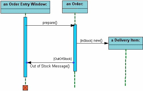
The next diagram shows the beginning of a sequence diagram for placing an order.  The object an Order Entry Window is created and sends a message to an Order object to prepare the order. Notice the the names of the objects are followed by a colon.  The names of the classes the objects belong to do not have to be listed.  However the colon is required to denote that it is the name of an object following the objectName:className naming system.

Next the Order object checks to see if the item is in stock and if the [InStock] condition is met it sends a message to create an new Delivery Item object.

The next diagrams adds another conditional message to the Order object.  If the item is [OutOfStock] it sends a message back to the Order Entry Window object stating that the object is out of stack.  

This simple diagram shows the sequence that messages are passed between objects to complete a use case for ordering an item.

Collaboration diagrams

Collaboration diagrams are also relatively easy to draw.  They show the relationship between objects and the order of messages passed between them.  The objects are listed as icons and arrows indicate the messages being passed between them. The numbers next to the messages are called sequence numbers.  As the name suggests, they show the sequence of the messages as they are passed between the objects.  There are many acceptable sequence numbering schemes in UML.  A simple 1, 2, 3... format can be used, as the example below shows, or for more detailed and complex diagrams a 1, 1.1 ,1.2, 1.2.1... scheme can be used.   

The example below shows a simple collaboration diagram for the placing an order use case.  This time the names of the objects appear after the colon, such as :Order Entry Window following the objectName:className naming convention. This time the class name is shown to demonstrate that all of objects of that class will behave the same way.

State Diagrams

State diagrams are used to describe the behavior of a system.  State diagrams describe all of the possible states of an object as events occur.  Each diagram usually represents objects of a single class and track the different states of its objects through the system. 

When to Use:

Use state diagrams to demonstrate the behavior of an object through many use cases of the system.  Only use state diagrams for classes where it is necessary to understand the behavior of the object through the entire system.  Not all classes will require a state diagram and state diagrams are not useful for describing the collaboration of all objects in a use case.  State diagrams are other combined with other diagrams such as interaction diagrams and activity diagrams.

How to Draw: 

State diagrams have very few elements. The basic elements are rounded boxes representing the state of the object and arrows indicting the transition to the next state. The activity section of the state symbol depicts what activities the object will be doing while it is in that state.   

All state diagrams being with an initial state of the object.  This is the state of the object when it is created.  After the initial state the object begins changing states.  Conditions based on the activities can determine what the next state the object transitions to.

Below is an example of a state diagram might look like for an Order object.  When the object enters the Checking state it performs the activity "check items."  After the activity is completed the object transitions to the next state based on the conditions [all items available] or [an item is not available].  If an item is not available the order is canceled.  If all items are available then the order is dispatched.  When the object transitions to the Dispatching state the activity "initiate delivery" is performed.  After this activity is complete the object transitions again to the Delivered state.

State diagrams can also show a super-state for the object. A super-state is used when many transitions lead to the a certain state.  Instead of showing all of the transitions from each state to the redundant state a super-state can be used to show that all of the states inside of the super-state can transition to the redundant state.  This helps make the state diagram easier to read.

The diagram below shows a super-state.  Both the Checking and Dispatching states can transition into the Canceled state, so a transition is shown from a super-state named Active to the state Cancel.  By contrast, the state Dispatching can only transition to the Delivered state, so we show an arrow only from the Dispatching state to the Delivered state.  

Activity Diagrams

Activity diagrams describe the workflow behavior of a system.  Activity diagrams are similar to state diagrams because activities are the state of doing something.  The diagrams describe the state of activities by showing the sequence of activities performed.  Activity diagrams can show activities that are conditional or parallel.

When to Use: 

Activity diagrams should be used in conjunction with other modeling techniques such as interaction diagrams and state diagrams.  The main reason to use activity diagrams is to model the workflow behind the system being designed.  Activity Diagrams are also useful for: analyzing a use case by describing what actions need to take place and when they should occur; describing a complicated sequential algorithm;  and modeling applications with parallel processes.

However, activity diagrams should not take the place of interaction diagrams and state diagrams.  Activity diagrams do not give detail about how objects behave or how objects collaborate. 

How to Draw: 

Activity diagrams show the flow of activities through the system.  Diagrams are read from top to bottom and have branches and forks to describe conditions and parallel activities.  A fork is used when multiple activities are occurring at the same time.  The diagram below shows a fork after activity1. This indicates that both activity2 and activity3 are occurring at the same time.  After activity2 there is a branch. The branch describes what activities will take place based on a set of conditions.  All branches at some point are followed by a merge to indicate the end of the conditional behavior started by that branch. After the merge all of the parallel activities must be combined by a join before transitioning into the final activity state.   

Below is a possible activity diagram for processing an order.  The diagram shows the flow of actions in the system's workflow.  Once the order is received the activities split into two parallel sets of activities.  One side fills and sends the order while the other handles the billing.  On the Fill Order side, the method of delivery is decided conditionally.  Depending on the condition either the Overnight Delivery activity or the Regular Delivery activity is performed.  Finally the parallel activities combine to close the order.  

Physical Diagrams

There are two types of physical diagrams: deployment diagrams and component diagrams.  Deployment diagrams show the physical relationship between hardware and software in a system.  Component diagrams show the software components of a system and how they are related to each other.  These relationships are called dependencies.

When to Use:

Physical diagrams are used when development of the system is complete.  Physical diagrams are used to give descriptions of the physical information about a system.  

How to Draw:

Many times the deployment and component diagrams are combined into one physical diagram.  A combined deployment and component diagram combines the features of both diagrams into one diagram.  

The deployment diagram contains nodes and connections.  A node usually represents a piece of hardware in the system.  A connection depicts the communication path used by the hardware to communicate and usually indicates a method such as TCP/IP.  

The component diagram contains components and dependencies. Components represent the physical packaging of a module of code. The dependencies between the components show how changes made to one component may affect the other components in the system. Dependencies in a component diagram are represented by a dashed line between two or more components. Component diagrams can also show the interfaces used by the components to communicate to each other.

The combined deployment and component diagram below gives a high level physical description of the completed system. The diagram shows two nodes which represent two machines communicating through TCP/IP. Component2 is dependant on component1, so changes to component 2 could affect component1. The diagram also depicts component3 interfacing with component1. This diagram gives the reader a quick overall view of the entire system.